In 1973, Fischer Black and Myron Scholes solved a problem that had stumped financial mathematicians for decades: how do you fairly price the right to buy a stock at a fixed price in the future?
Their answer was the Black-Scholes formula which is now used millions of times a day on trading floors around the world. In this section I’m going to build it from scratch in Python and apply it to Apple’s stock in real time.
I utilised a variety of different python libraries to obtain the results. Y finance was used to obtain real time data of the stocks. In this case I used Apple stock data for the year 2025. Numpy was used for the calculations as it can perform optimised mathematical operations on large arrays. I also used MatPlot for the creation of the graph which I will add in towards the end. It allows you to customise the graph and is a neat way of illustrating the data.
So with the use of Y Finance I was able to extract real world data. In the case of Apple the historical volatility was 31.7% calculated from a full year of returns.
The Inputs:
To price an option you need the following 5 inputs:
S – The current stock price
K – The strike price
T – The time to expiry in years
r – The risk free interest rate
σ – The volatility i.e. how much the stock price moves around.
As mentioned previously I obtained the first 2 through the Y finance library. Apple was trading at $253.92 at the time of making this. The volatility was calculated based on a full year of returns. As the Apple stock had been moving around quite a lot the volatility was annualised at around 31%. The volatility is relatively high and demonstrates the choppy period the market is currently in. I calculated the strike price at the money which is relatively common.
The formula has two components. The first S * norm.cdf(d1) —represents what you expect to receive: the asset, if the option finishes in the money. The second K * exp(-rT) * norm.cdf(d2) is what you’ll pay: the strike price, discounted back to today. The difference between them is the fair value of the option.
With Apple at $253.92 and volatility at 31.7%, the model prices a six-month at-the-money call at $25.63.
Volatility is the biggest driver. Dropping volatility from the real 31.7% down to 20% collapsed the option price from $25.63 to just $8.02 — a two-thirds reduction with the stock price completely unchanged. This is what the Greek called Vega measures: how much the option price moves per 1% change in volume.
The strike determines money. Moving the strike from $254 to $270 taking the option out of the money dropped the price from $25.63 to $16.00. The stock would need to rally more than 6% before the option becomes profitable at expiry, so the market charges less for it.
The stock price moves the option in real time. Between my first run of the code and my second, Apple moved from $247.99 to $253.92. The option price moved from $25.09 to $25.63 in response. That ratio how much the option moves per $1 move in the stock is Delta, and observing it live makes the concept immediately tangible.
Rather than pricing the option at a single stock price, I priced it across every hypothetical stock price from $180 to $320 and plotted the result.
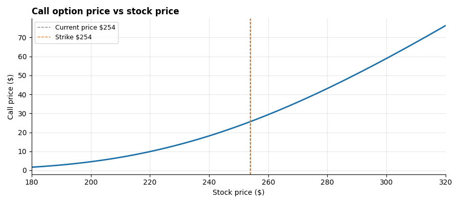
The shape of this curve tells you almost everything about how options behave. When Apple is deep below the strike the option is nearly worthless, there is almost no chance of it finishing profitably. As the stock approaches the strike the curve steepens sharply: small moves in the stock produce large moves in the option price. This steepening is Gamma. Deep above the strike, the curve flattens again and the option moves nearly one-for-one with the stock, Delta approaching 1.
Options traders are running this calculation thousands of times a day, adjusting for real-time price and volatility changes across entire books of positions. Understanding the model from first principles, not just using it as a black box, is what separates a trader who manages risk from one who merely takes it.
Building it in Python, connected to live market data, makes that understanding concrete rather than theoretical.
